Sabina’s Stats Corner: Mastering the Normal Distribution and Central Limit Theorem

Special Notes:

Listen to our L&L lectures online: WHRI Lunch & Learn Series – Women’s Health Research Institute

Visit our Stats corner in the e-blast for previously published tips on data management and analysis: E-Blast Archive – Women’s Health Research Institute (whri.org)

Normal Distribution Summary

During our “Sabina’s Stats Series” lecture on September 28th, 2023, we discussed statistical distributions and their applications. I emphasized the significance of the Central Limit Theorem (CLT), a fundamental theorem in probability theory, several times throughout the lecture. This newsletter aims to summarize the importance of this theorem in statistics and its practical utility.

The normal distribution is exceedingly important because it manifests ubiquitously in the real world. Imagine having a substantial dataset, such as people’s heights or test scores. When plotted on a graph, this data often forms a symmetrical, bell-shaped curve. This curve aids in understanding and predicting trends within the data.

What’s remarkable about the normal distribution are its special properties. For instance, it facilitates determining the likelihood of various outcomes and aids in decision-making based on probabilities. It serves as a valuable tool for scientists, statisticians, and researchers to comprehend a wide array of data, from predicting the likelihood of rain on a given day to estimating the probability of achieving a certain grade on a test. Simply put, the normal distribution acts as a friendly guide, enhancing our comprehension and manipulation of data.

What is the Central Limit Theorem (CLT)?

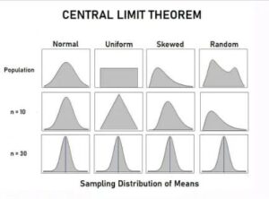
The Central Limit Theorem operates akin to a magical recipe for transforming messy data into a neatly structured, normal-looking graph (bell curve). Envision having an assortment of random entities, such as people’s heights or test scores. By aggregating numerous instances and calculating their average, the resulting distribution increasingly resembles a bell curve as the sample size grows. This process transforms chaos into order, thereby enhancing our understanding and utilization of data.

In probability theory, the CLT asserts that the distribution of a sample variable approximates a normal distribution (i.e., a “bell curve”) as the sample size increases. This holds true regardless of the actual shape of the population’s distribution, assuming all samples are identical in size.

Brief Historical Facts – An International Collaboration of Brilliant Mathematicians Over Multiple Years

The development of the Central Limit Theorem was a collaborative endeavor involving numerous mathematicians and statisticians spanning centuries. It has profoundly impacted various fields, including statistics, economics, and natural sciences, by furnishing a potent tool for comprehending the behavior of sums of random variables.

Early Concepts (18th Century):

The concepts underlying the CLT began to surface in the 18th century. Mathematicians such as Abraham de Moivre and Pierre-Simon Laplace delved into the distribution of sums of independent and identically distributed (i.i.d.) random variables.

Laplace's Work (1810):

Pierre-Simon Laplace made significant contributions by formulating an early version of the CLT. He explored the limiting distribution of the binomial distribution as the number of trials increased substantially.

Gauss and the Normal Distribution (19th Century):

Carl Friedrich Gauss, often regarded as one of the greatest mathematicians, developed the normal distribution and made invaluable contributions to probability theory. Although he did not explicitly state the CLT, his work laid the groundwork for its eventual formulation.

Chebyshev's Inequality (1867):

The Russian mathematician introduced Chebyshev’s inequality, which provided bounds on the probability of deviations from the mean. While not directly linked to the CLT, it played a role in its evolution.

Lyapunov's Contribution (1901):

The Russian mathematician made significant strides in the development of the CLT by establishing conditions under which it holds true. He extended the concept of convergence in distribution.

Modern Formulation (1920s):

The modern formulation of the CLT, as known today, was refined in the early 20th century by multiple statisticians, including Aleksandr Khinchin and Harald Cramér. They elucidated and refined the conditions necessary for the theorem’s applicability.

Lindeberg's Contributions (1922):

The Swedish mathematician provided crucial insights into the CLT, focusing on convergence rates and the conditions under which the CLT holds for samples of varying sizes.

Emil Borel's Theorem (1925):

The French mathematician independently contributed to the CLT. His theorem posited that the normal distribution is the sole limiting distribution for standardized sums of independent random variables with finite variances.

Central Limit Theorem in Textbooks (Mid-20th Century):

The CLT became a cornerstone topic in statistics and probability theory, finding its way into textbooks and becoming a standard tool for statisticians and scientists.

How to Use CLT

Let’s consider you work at a candy factory, responsible for ensuring the candy bars have accurate weights. Recognizing that the machines producing the candy bars may exhibit slight variations, resulting in non-uniform weights, here’s how you can apply the Central Limit Theorem in this scenario:

Collect Data: Begin by individually weighing numerous candy bars to gather a sample of weights.

Calculate the Average: Determine the average weight of the candy bars within your sample.

Repeat: Iterate this process multiple times, weighing different batches of candy bars each time and computing the average weight for each batch.

Create a Histogram: Construct a histogram, akin to a bar chart, illustrating the frequency of occurrence for each average weight.

Apply the Central Limit Theorem: In accordance with the CLT, with a sufficiently large number of samples and adequately sized samples, the histogram of these sample averages will begin to resemble a bell curve (normal distribution).

Make Predictions: Utilizing this bell curve, you can now make predictions, such as estimating the percentage of candy bars falling within a specific weight range or establishing quality control thresholds to ensure most candy bars meet the desired weight criteria

Additional Examples:

Good luck with your Statistics adventure!

Contact Sabina for statistics help or questions here: sabina.dobrer@cw.bc.ca