Special Notes:
Listen to our L&L lectures online: WHRI Lunch & Learn Series – Women’s Health Research Institute
Visit our Stats corner in the e-blast for previously published tips on data management and analysis: E-Blast Archive – Women’s Health Research Institute (whri.org)
Check out our new YouTube channel for insightful presentations and resources:
If you’re new to WHRI, my two Lunch and Learn lectures are helpful for grasping basic analytical concepts:
Data Cycle and Use of Data in Research:Data Life Cycle (YouTube)
Philosophical Concepts of Statistics and Uncertainty: Lunch and Learn 4: What is Stats? A Series of Un/fortunate Events (YouTube)
My previous statistics lectures are available here:
Sabina’s Stats Series – YouTube
For a deep dive into data visualization, check out my Summer Scholar lecture:
Welcome!
We’re back! In one of my first lectures, we covered the basics of probability and statistical uncertainty, discussing how uncertainty arises from incomplete information and inherent unpredictability. A key type, Aleatory Uncertainty, reflects the natural randomness in our data, like rolling a die. This uncertainty, embedded in our measurements and sampling process, is captured in the error term.
In short, statistical uncertainty is always present, reminding us we’re working with probabilities, not certainties—keeping things interesting!
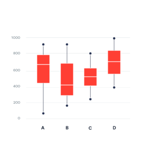
When reporting results, it’s important to incorporate uncertainty, and one way is through confidence intervals (CI). CIs provide context by showing a range of possible outcomes, helping ensure our findings are transparent, trustworthy, and statistically sound.
In statistics, we rarely know the “true” population, so we use CIs to estimate where population parameters, like the mean, likely fall. For example, a 95% confidence interval means we can be 95% certain the true population mean lies within that range. The p-value, often set at 5%, tells us the risk of making a Type I error—rejecting a true null hypothesis.
Example of CI Calculation
Here’s a simple example using the normal distribution (“bell curve”) to calculate a 95% confidence interval for the average height of adults in a city, based on a sample of 100 people.
Mean (sample estimate): 170 cm
Standard error: 10 cm
Sample size: 100
Confidence level: 95%
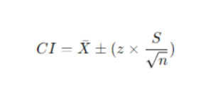
Since 95% of the data in a normal distribution lies within 1.96 standard deviations (z-score), we can apply the formula for calculating CI:
Calculation:
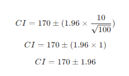
Interpretation:
This means we are 95% confident that the true average height of all adults in the city lies between 168.04 cm and 171.96 cm. The tails of the normal distribution indicate that only 5% of the time (2.5% in each tail), the true mean would fall outside this range.
This is how confidence intervals offer a clear range that reflects the uncertainty in our sample estimate, using the normal distribution’s tails to guide us!
Good luck with your Statistics adventure!
Contact Sabina for statistics help or questions here: sabina.dobrer@cw.bc.ca